
Many public discussions of AI ask how much more a model can do when we give it more: more parameters, more memory and more computing power. Geisten asks the opposite question: how small can a useful AI system become?
BitNet is an interesting test case because its weights have only three values: −1, 0 and +1. They can be packed densely, reducing the amount of model data a CPU must move from memory. Specialized kernels can also replace many general weight multiplications with additions, subtractions or efficient integer dot products. This creates room for CPU optimization, although it does not make the complete model multiplication-free or automatically energy-efficient.
A Raspberry Pi 5 is a good place to make that question concrete. It is small, inexpensive and limited to a CPU and 4 GB of memory in this experiment. There is nowhere for inefficient software to hide. If a two-billion-parameter language model runs well here, we can inspect which design choices make that possible—and which limits remain.
This experiment asks whether those constraints still leave enough room for useful local inference. It is not an attempt to rebuild a cloud assistant on a tiny computer. It is a first step toward understanding the basic ingredients of local AI: enough speed for interaction, low enough memory use to fit, modest power demand and sufficient model quality for a defined task.
I wrote geistlib, a small inference engine in C, to make those ingredients easier to inspect. General-purpose runtimes must support many models and machines. geistlib deliberately supports less. That narrower scope lets me change one implementation detail, measure the result and keep the deployment simple. It is a laboratory instrument, not a finished assistant.
Research question: what the measurements are for
The central question is whether a specialized runtime can execute BitNet 2B-4T usefully on a 4 GB Raspberry Pi 5. “Usefully” is too vague to measure directly, so the experiment breaks it into five smaller questions:
| Reader question | Why measure it? | Evidence used here |
|---|---|---|
| Does the model respond fast enough for interaction? | A model that fits but answers too slowly is not practically local. | Decode throughput |
| Does specialization help? | A standalone speed number says little without a comparable implementation. | Same-model bitnet.cpp baseline |
| How much speed is still available? | This separates obvious software overhead from a hardware limit. | Measured memory roofline |
| What does inference appear to consume inside the board? | Edge hardware needs a measurable power budget. | Internal PMIC telemetry, with no total USB-C power claim |
| Is the model’s output useful? | Fast nonsense is still nonsense. | MMLU sample and informal language probes |
These measurements do not produce a single verdict. Together they show where this prototype already works, where the hardware sets a boundary and what still needs a better experiment.
A first answer from the Pi
On a supported Linux or macOS system, the quickest installation is:
curl -fsSL https://raw.githubusercontent.com/geisten/geistlib/main/install.sh | sh
The download is large—about 1.1 GB—because the BitNet model is bundled inside
the geist-bitnet executable. After installation there is no separate model
file to find and no Python, CUDA, BLAS or Docker runtime to configure. On Linux,
the released program is a statically linked single file.
I began with the simplest visible test I could think of:
$ geist-bitnet "What is the capital of France?"
The capital of France is Paris
Across five new processes with the Linux filesystem cache cleared before each run, the complete command took about 3.4 seconds. This includes loading the embedded model, processing the prompt, generating the answer and printing it. It is an end-to-end startup measurement, not time to first token.
The answer is not surprising. Where it came from is more interesting: the model and the inference engine ran entirely on the Pi.
Under the tested setup, geistlib generated about 18 tokens/s. A memory measurement puts an optimistic ceiling at about 22 tokens/s for this particular decode path. Internal power sensors reported an average of 5.9 W during a longer run. But those sensors do not see everything that enters through the USB-C connector, so 5.9 W is not the Pi’s total power consumption. We will record the exact usage with a measuring device for a future article.
That short answer is only the entrance to the experiment. The remaining sections test how fast the engine is, why it reaches that speed, what the power sensors can actually tell us and where the model’s quality falls short.
Why build another inference engine?
The main reason was to learn. Implementing model loading, quantization and CPU kernels from scratch made the algorithms visible: I could change one step, measure the effect and understand why it helped or failed. The performance numbers are evidence from that learning process, not the original reason for starting another runtime.
General-purpose runtimes support many models and platforms. That breadth has a cost on constrained hardware, while a narrower experimental engine can focus on a few paths.
In one documented Raspberry Pi test, stock Ollama 0.30.10 was killed while
loading Gemma 4 E2B on a 4 GB board. A 1.93 GB internal table was copied into
resident memory. Enabling use_mmap and reducing the batch size made the model
load. geistlib maps this table from the model file by default.
This does not show that Ollama is generally inefficient. It shows that memory policy can decide whether one specific model starts on a 4 GB machine. The full setup and the corrected thermal methodology are recorded in the Raspberry Pi benchmark.
geistlib 0.5.0 is experimental and supports much less than llama.cpp. The project is useful here because its narrow scope makes individual design choices measurable.
Experimental setup
The throughput measurements used:
- Raspberry Pi 5 Model B Rev 1.1
- four Cortex-A76 cores and 4 GB RAM
- 64-bit Raspberry Pi OS, Debian, Linux kernel 6.18
- performance governor at 2.4 GHz
- a cool, idle board, recorded at 45 °C for the BitNet run
- geistlib 0.5.0
- Microsoft BitNet b1.58 2B-4T, canonical
i2_sGGUF, 1.19 GB - greedy decoding with the speculative output head enabled
- two threads for the reported 17.580 tokens/s result
bench_perf_sweep ran five measured repetitions after a discarded warm-up.
The bitnet.cpp comparison used the same Pi, model and greedy decoding. A new
audited run pins Microsoft BitNet commit
01eb415772c342d9f20dc42772f1583ae1e5b102 and its bundled llama.cpp
submodule at 1f86f058de0c3f4098dedae2ae8653c335c868a1.
Ternary inference on the Pi
Why choose a ternary model for this experiment? On the Raspberry Pi, memory bandwidth is a hard constraint. Moving billions of model weights through memory can therefore matter as much as the arithmetic itself.
BitNet b1.58 restricts each weight to three possible values: −1, 0 and +1. That makes the weights compact and gives the inference engine simpler integer operations to work with. It does not make the complete model multiplication-free, and it does not prove that the finished system uses less energy. Those questions still require measurements.
The ternary design was introduced in
The Era of 1-bit LLMs, while the tested
2B-4T checkpoint is described in its
technical report. geistlib’s ARM path uses
SDOT integer dot products and defers the −1 bias correction. The published Pi
result uses the canonical i2_s model.
A later base-three packing stores five ternary values per byte and improved decode by 10.5 percent in an AMD Ryzen 9 9950X ablation. That is an x86 result, not the explanation for the Pi number.
On the Pi, profiling identified the tied F16 output head as roughly half of baseline decode time. geistlib builds a smaller int8 sketch to select candidate tokens, then computes exact F16 logits for those candidates. Across the reported probes, greedy output matched the dense head byte for byte. The v0.5.0 release uses a stride of four and retains 1,024 candidates for exact F16 rescoring. With this path enabled, the earlier development measurement increased from 9.83 to 17.4 tokens/s.
Measured throughput
The first practical test is response speed. I compare geistlib with bitnet.cpp because both can execute the same BitNet model on the same Pi. This does not rank either project in general; it tests whether geistlib’s narrow implementation helps on this one path.
| System | Metric | geistlib | bitnet.cpp | Ratio |
|---|---|---|---|---|
| Raspberry Pi 5 | Decode, low context | 17.580 tokens/s | 9.139 tokens/s | 1.92× |
| AMD Ryzen 9 9950X | Decode, 128 tokens | 103.1 tokens/s | 54.3 tokens/s | 1.90× |
The geist value in the Pi row is a new mean of five measured runs after a discarded 32-token prefill and four decode steps, using two threads. It was built directly from the published v0.5.0 tag. The measured range was 17.567 to 17.598 tokens/s, calculated from the best and worst recorded decode times. The commit-pinned bitnet.cpp value is a mean of ten four-thread runs, its fastest measured thread configuration. The same bitnet.cpp run produced 8.233 tokens/s with two threads, reproducing the earlier rounded 8.2 tokens/s observation. The x86 rows use mean-of-five measurements with 16 physical cores. The detailed geist protocols and negative results are in the ternary Pi log and x86 benchmark. The new bitnet.cpp raw results preserve commands, per-run samples, source revisions and artifact hashes. The version-pinned Pi rerun is preserved in the roofline run and its manifest.
These measurements show geistlib ahead of the tested bitnet.cpp build on these three paths. They do not establish a general lead across models, runtimes or hardware.
How close is decode to the hardware limit?
A faster baseline result does not tell us whether another small optimization could double the speed or whether the Pi is already close to its limit. To separate those possibilities, I estimated two ceilings: how quickly the Pi can read the required model data, and how quickly its CPU can perform the required integer operations. The lower ceiling is the useful one.
This calculation is a low-context decode roofline: an optimistic upper bound derived from compulsory model traffic, measured sequential-read bandwidth and the processor’s documented SDOT issue rate. The method follows the separation of memory and compute ceilings in the Roofline model.
The scope is single-batch greedy decode with two threads and the v0.5.0 speculative output head. It does not apply directly to prefill. Prefill reuses weights across multiple input tokens and has different matrix shapes and operational intensity.
Minimum bytes per generated token
Before comparing decode with memory speed, we need to estimate how much model data the engine must read for one new token. Even a perfect implementation cannot avoid these compulsory reads.
The GGUF metadata reports 30 layers, hidden size 2,560, intermediate size 6,912, 20 query heads, five key/value heads and a vocabulary of 128,256. From those dimensions and the release implementation, the minimum compulsory reads for one generated token are:
| Component | Derived bytes/token |
|---|---|
| Packed two-bit attention and FFN weights | 521,011,200 |
| F32 normalization weights | 1,761,280 |
| Stride-four int8 vocabulary sketch | 82,083,840 |
| Per-row sketch scales | 513,024 |
| 1,024 exact F16 candidate rows | 5,242,880 |
| Minimum total | 610,612,224 |
This 610.612 MB value is a calculated lower bound, not measured DRAM traffic. It assumes each listed weight byte is fetched once and does not add cache-line overfetch, page-table traffic, activation spills, OpenMP overhead, weight unpacking, non-matrix operations or context-dependent KV-cache traffic.
Memory ceiling
The memory ceiling asks a simple question: if each token requires at least 610.612 MB of model data, how many such chunks can the Pi’s memory deliver per second?
Raspberry Pi documents a 32-bit LPDDR4X interface with up to 17 GB/s of memory bandwidth. Dividing that interface rating by the minimum byte count gives a physical, unattainable-in-practice ceiling of 27.841 tokens/s.
I also measured a simpler sustained-read workload on the same board. It read a 512 MiB buffer after two discarded warm-ups, with ten measured repetitions, the performance governor at 2.4 GHz and no recorded throttling. At the thread-matched count of two, median bandwidth was 13.612 GB/s, with a range of 13.364 to 13.749 GB/s. That produces a more useful, but still optimistic, memory ceiling:
13.611852 GB/s / 0.610612224 GB/token = 22.292 tokens/s
The raw one-, two- and four-thread samples are
archived here,
and the exact calculation is in
derived-roofline.json.
Compute ceiling
Memory is not the only possible bottleneck. The CPU must also process the weights after reading them. A separate compute ceiling checks whether the processor’s arithmetic capacity is lower than the memory limit.
Arm’s Cortex-A76 optimization guide specifies a maximum throughput of two 128-bit SDOT instructions per cycle. Each instruction performs 16 int8 multiply-accumulates. At 2.4 GHz and two threads, that gives an optimistic peak of 153.6 billion int8 multiply-accumulates per second.
The ternary layers and vocabulary sketch require an estimated 2.166 billion int8 multiply-accumulates per generated token. Dividing the instruction peak by that work gives 70.910 tokens/s. The four-core instruction ceiling would be 141.820 tokens/s. Both are far above the measured memory ceiling, even before accounting for the instructions required to unpack two-bit weights. The roofline therefore identifies memory traffic, not raw SDOT capacity, as the tighter theoretical limit for this decode path.
The immediate conclusion is that more arithmetic alone is unlikely to transform this decode path. A platform with higher sustained memory bandwidth could benefit more, provided its caches and kernels can keep the data moving. The gain would not necessarily scale in direct proportion to bandwidth: unpacking, attention, synchronization and the output head would eventually become the next limits.
Interpreting 17.580 tokens/s
The lower-bound traffic at the measured rate corresponds to at least 10.735 GB/s:
17.580 tokens/s × 0.610612224 GB/token = 10.735 GB/s
The observed 17.580 tokens/s is 78.9 percent of the 22.292-token/s sustained read roofline and 63.1 percent of the 27.841-token/s interface-rating ceiling. This does not mean the engine uses exactly 78.9 percent of DRAM bandwidth. The numerator uses a compulsory-byte lower bound, while the denominator comes from a simpler sequential-read loop. The remaining gap includes weight unpacking, attention, normalization, candidate selection, synchronization and less ideal memory access. The experiment does not isolate their individual shares.
The defensible conclusion is that low-context decode is already operating in the memory-bound region and within roughly one fifth of this measured sequential-read roofline. It is not evidence that 22.292 tokens/s is achievable by the complete engine, nor does it establish a theoretical prefill limit.
Deployment scope
Local AI is not only a question of benchmark speed. If installation needs a large software stack or a model cannot travel with the program, deployment on small devices becomes harder.
geistlib can build without Python, CUDA, BLAS or Docker. Linux supports a static musl build, while macOS uses system frameworks. A model can be embedded into the executable, and GPU backends are loaded at runtime rather than linked as mandatory dependencies.
This is a deployment property, not a quality metric. A smaller runtime also supports fewer models, formats and hardware paths than llama.cpp.
The quick-start installer follows the latest release. For a reproducible research setup, use the v0.5.0 release artifacts instead of relying on that moving target.
What the PMIC measurement tells us
Throughput and compact weights do not establish energy efficiency. We need a power measurement to learn whether the Pi draws modest power while it is actually generating text. The board exposes internal sensors for this purpose, but they see only part of the electrical path.
The test used a Raspberry Pi 5 with 4 GB RAM, geistlib 0.5.0, the
canonical BitNet 2B-4T i2_s model and four threads. It ran one excluded
warm-up followed by ten measured repetitions. Each repetition processed 32
prefill tokens and generated 256 decode tokens.
Every 200 ms, the measurement script called vcgencmd pmic_read_adc and
stored the unmodified output with a monotonic timestamp, temperature, ARM
clock and throttling state. For each named rail that exposed both current and
voltage, the derived analysis calculated:
PMIC rail-sum proxy = Σ (rail current × rail voltage)
The sum is deliberately named a proxy. It is a derived view of the PMIC’s internal rail telemetry, not a direct reading at the board’s power connector.
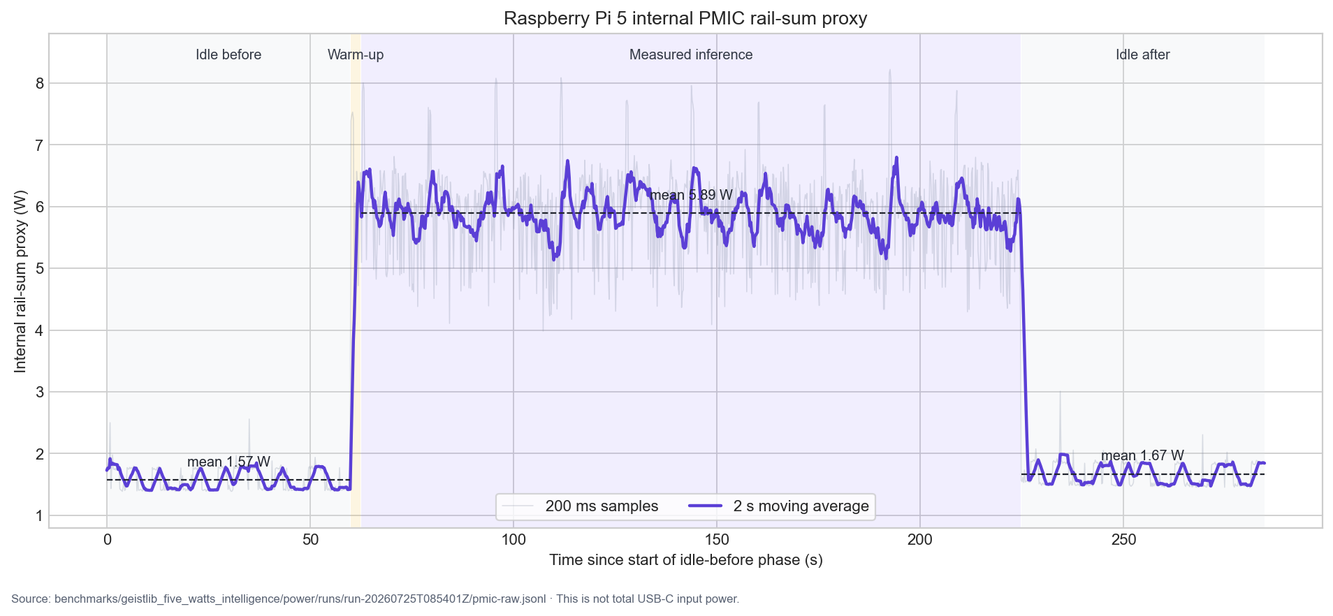
The 200 ms samples and a two-second moving average show the change between idle and inference. Dashed lines mark the phase means. Source: archived raw PMIC trace. This is not total USB-C input power.
Repeated measurement
| Phase | Samples | Duration | Mean proxy | Median proxy | Integrated proxy |
|---|---|---|---|---|---|
| Idle before | 300 | 59.822 s | 1.573 W | 1.440 W | 94.107 J |
| Measured inference | 810 | 161.985 s | 5.889 W | 6.051 W | 954.226 J |
| Idle after | 300 | 59.822 s | 1.671 W | 1.556 W | 99.927 J |
The inference process generated 2,560 decode tokens. Dividing the integrated inference proxy by that count gives:
954.226 J / 2,560 generated tokens = 0.373 J/token
This gross value includes the prefill phase of each repetition in the energy numerator. Subtracting the mean of the two idle baselines gives an exploratory dynamic proxy of 0.270 J per generated token. Both numbers remain PMIC-derived proxies.
The same session reported 16.475 decode tokens/s with four threads. Temperature
rose from 52.7 to 68.6 °C, the ARM clock remained near 2.4 GHz, and every
captured throttling value was 0x0. This power run is separate from the
two-thread, 17.580 tokens/s throughput comparison earlier in the article.
What would this mean for a 10,000 mAh power bank? The label alone is not enough; voltage and conversion losses matter. If the rating means 10,000 mAh at 3.7 V, the pack stores 37 Wh nominally. With 85 percent usable after conversion, a hypothetical USB-C load of 6 to 8 W would run for roughly 3.9 to 5.2 hours. That is a scenario, not a result from this experiment, because actual USB-C input power was not measured.
What the 5.9 W number means
The internal trace is useful for comparing runs on the same board. It can show, for example, whether an optimization shortens the time spent at high internal power. It cannot establish the Pi’s absolute input consumption.
Raspberry Pi’s own documentation states that pmic_read_adc cannot see USB
current or other devices connected directly to 5 V because those paths bypass
the PMIC. It explicitly warns that the readings should not be expected to add
up to the wattage of the source power supply. The command exposes EXT5V_V,
the external 5 V supply voltage, but not the corresponding total input
current. See the
Raspberry Pi PMIC documentation.
The rail sum also excludes conversion losses between the USB-C input and the regulated outputs. This experiment did not validate each ADC channel against a calibrated instrument, so there is no measured correction factor. An inline USB-C analyzer or calibrated bench supply is needed for that number. The derived phase summary preserves the exact PMIC values used here.
Quality: what the model knows and what it does not
The runtime can make a model faster, but it cannot make the model know more. That is why speed and power need a separate quality check. MMLU provides a limited test of multiple-choice knowledge; it does not tell us whether the model can operate tools or follow instructions reliably.
The audited MMLU run records 207 correct answers out of 400, or 51.75 percent, with five examples in each prompt. Random guessing would yield 25 percent. The first 200 selected items produced 100 correct answers, exactly reproducing both historical aggregate outputs.
The replacement run preserves all 400 individual predictions. Each JSONL
record includes the original cais/mmlu test index, question, choices, gold
answer, predicted answer, four answer log-probabilities, prompt-token count,
prompt hash and the five development-set examples used in the prompt. Its
manifest records the complete command line, dataset fingerprints, shuffle seed,
BOS token, model checksum, evaluator checksum and source revision.
The primary evidence is the audited MMLU result, per-item predictions and run manifest. The earlier aggregate-only files remain preserved as historical evidence: 400-question results and 200-question results.
A separate documented Gemma 4 E2B run scored 89/200, or 44.5 percent. The question selections were not shown to be identical, and the sample sizes differ. These measurements therefore do not establish that BitNet is better than, equal to or non-inferior to Gemma. They only show the observed scores for the two recorded samples.
The BitNet sample produced the following grouped results:
| Subject group | Correct | Accuracy |
|---|---|---|
| Humanities and social knowledge | 73/106 | 68.9% |
| Medicine and biology | 33/62 | 53.2% |
| Psychology, ethics and applied law | 66/135 | 48.9% |
| Science, mathematics, chemistry and accounting | 35/97 | 36.1% |
The 200-question sample showed the same ordering. This is an observation about these samples. It does not prove that the model “knows facts but cannot reason,” and it does not demonstrate summarization, intent recognition, tool selection or home-control accuracy. Those remain hypotheses for task-specific evaluation.
Four informal language probes also produced much better English than German. For example:
$ geist -m bitnet-2b4t-i2_s.gguf "Was ist die Hauptstadt von Frankreich?"
Die Hauptstadt des Frankreichs ist derstadt Paris
Four prompts are enough to expose a practical warning, but not enough to measure language quality. The failure belongs to the model and prompt setup, not automatically to the engine.
Limitations
- Total power at the USB-C input has not been measured.
- PMIC ADC calibration error and the monitoring overhead were not measured.
- The power benchmark reports one aggregate result across ten internal repetitions; the PMIC trace does not delimit every repetition separately.
- The internal-rail proxy has not been compared with a calibrated external power instrument.
- Power and throughput used different thread configurations.
- The roofline uses a calculated lower bound of compulsory reads, not phase-isolated DRAM traffic from the inference process.
- The sequential-read microbenchmark has a simpler access pattern than geistlib and therefore provides an optimistic sustained ceiling.
- The theoretical calculation covers low-context decode, not prefill or long context. KV-cache traffic grows with context.
- The MMLU sample covers 400 of the dataset’s 14,042 test questions.
- The subject-group interpretation is exploratory.
- No task-specific accuracy test yet supports claims about summarization, classification, tool selection or home automation.
- geistlib 0.5.0 is experimental and covers fewer architectures and platforms than established runtimes.
Reproducibility
The source snapshot used for this article is
geistlib v0.5.0,
commit 393676cd472ecd5b1d64a5736002625127975883.
The documented Pi throughput command is:
make TARGET=pi5
bin/pi5/release/tests/bench_perf_sweep \
  --gguf /path/to/ggml-model-i2_s.gguf \
  --seq-lens 32,128,256 \
  --decode-n 64
Run it on a cool, idle Raspberry Pi 5 with the performance governor at 2.4 GHz. The audited runs linked below record the model checksum and the pinned bitnet.cpp revision.
The version-pinned Pi measurement used:
make TARGET=pi5 bin/pi5/release/tests/bench_perf_sweep -j4
OMP_NUM_THREADS=2 OMP_PROC_BIND=close OMP_PLACES=cores \
  bin/pi5/release/tests/bench_perf_sweep \
  --gguf /path/to/bitnet-2b4t-i2_s.gguf \
  --seq-lens 32 --decode-n 64 --warmup 32 \
  --repeats 5 --threads 2 --emit-jsonl
The release archive, binary and model hashes are recorded in the
roofline manifest.
The sustained-read benchmark and deterministic calculation are preserved as
stream_read.c
and
calculate_roofline.py.
The audited MMLU harness is preserved as
run_mmlu_audited.py.
The archived run used:
python3 run_mmlu_audited.py \
  --output-dir run-YYYYMMDDTHHMMSSZ \
  --bin /path/to/eval_geist \
  --gguf /path/to/ggml-model-i2_s.gguf \
  --source-repo /path/to/geistlib \
  --limit 400 --shots 5 --bos 128000 --seed 1234 \
  --dataset cais/mmlu --dataset-config all
The exact executed argument vector and normalized absolute command are in the
MMLU manifest.
The model SHA-256 is
4221b252fdd5fd25e15847adfeb5ee88886506ba50b8a34548374492884c2162.
The PMIC experiment is archived with its measurement script, manifest, benchmark output and raw JSONL trace. The manifest preserves the complete command, model and binary checksums, generated-token count, operating system, governor, temperatures and throttling state.
The chart in this article is generated from that unmodified JSONL trace by
plot_pmic_trace.py.
The embedded-model startup measurement, including all five cache-cold samples, the timing boundary and binary checksum, is preserved in the cold-start record.
The short response is archived with its complete manifest and ten measured outputs. The commit-pinned bitnet.cpp baseline includes its manifest and raw two- and four-thread benchmark outputs.
Sources
- Wang et al., BitNet: Scaling 1-bit Transformers for Large Language Models, 2023.
- Ma et al., The Era of 1-bit LLMs: All Large Language Models are in 1.58 Bits, 2024.
- Ma et al., BitNet b1.58 2B4T Technical Report, 2025.
- Wang et al., bitnet.cpp: Efficient Edge Inference for Ternary LLMs, 2025.
- Williams, Waterman and Patterson, Roofline: An Insightful Visual Performance Model for Floating-Point Programs and Multicore Architectures, 2008.
- Arm, Cortex-A76 Software Optimization Guide, version 10.0.
- Raspberry Pi, BCM2712 processor documentation.
What comes next
The next useful experiments are narrower than a product demo:
- measure USB-C input power alongside the existing PMIC logger
- compare the PMIC proxy with the external instrument across idle and load
- isolate inference-phase DRAM traffic with a phase-aware PMU or memory controller counter
- run task-specific tests for summarization, classification and tool routing
- compare models on identical MMLU questions and commands
The current evidence already shows that a specialized engine can run this ternary model at 17.580 tokens/s on a Raspberry Pi 5 under the documented conditions. It does not yet show which application should trust the model, or how much energy a reproducible deployment will consume at the wall.